My College Buildings Are More Historic Than Yours

Above: Old Main Building, South College Street,  Auburn, Alabama

In recently researching Southern Architecture, I came across the this nugget of information from Kenneth Severens in Southern Architecture: 350 Years of Distinctive American Buildings. As of the writing of the publication in 1982,  of the ten colleges designated in the National Historic Landmarks, seven were in the South.  Severens goes on to state that no section of the county has been more influential than the South in campus planning.  An interesting hypothesis indeed and one which is testable.

Below is a map of all of the buildings on university, college, and institute buildings listed on the National Register of Historic Places.

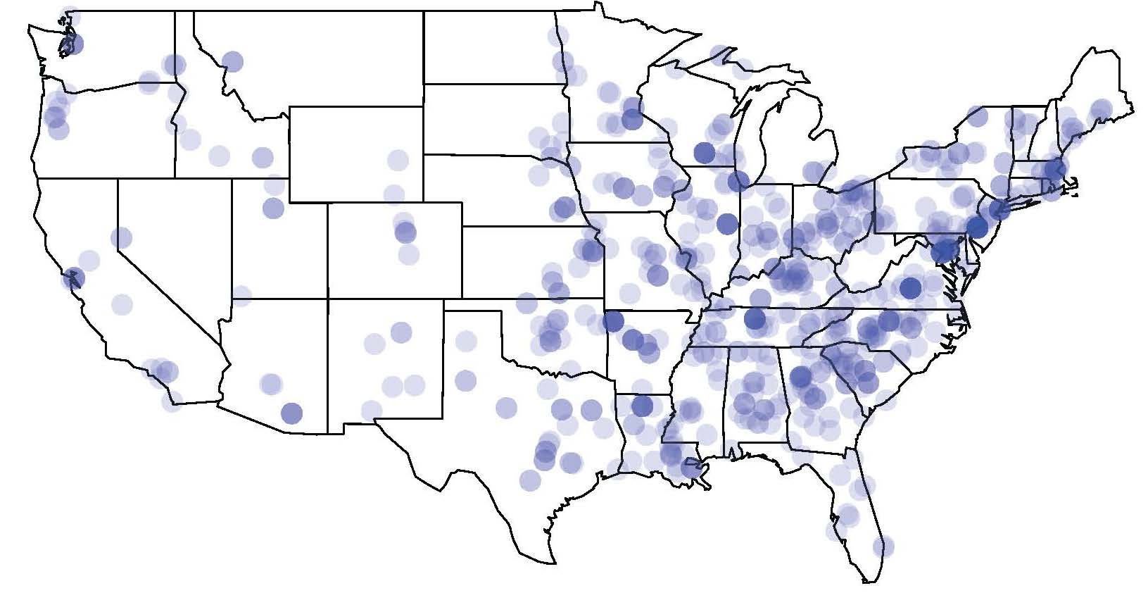
Clearly there does seem to be some concentration in South and particularly the Southeast. However, the number does not look much greater than that of Central Valley or New England.  Generating the boxplot below yields a clearer picture.

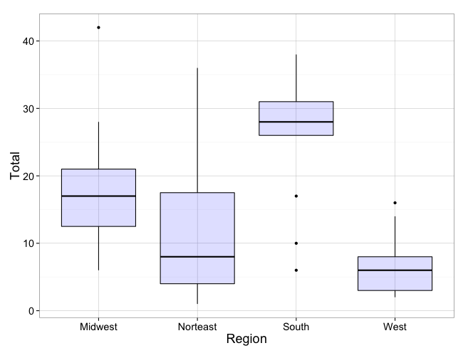
This yields a much clearer indication that Severens’ idea has merit.  A test of this however yields that the pattern for the South is just barely insignificant (p=0.06).  While the number per state for the West is significantly lower than the other sections (p=0.004).  The South is brought down by three slacker states–West Virginia, Florida, and Mississippi. That record holder for the Midwest? Ohio with 42.

South	WEST VIRGINIA	6
South	FLORIDA	10
South	MISSISSIPPI	17
South	ARKANSAS	26
South	VIRGINIA	26
South	ALABAMA	27
South	SOUTH CAROLINA	28
South	TEXAS	28
South	LOUISIANA	29
South	TENNESSEE	31
South	KENTUCKY	32
South	GEORGIA	34
South	NORTH CAROLINA	38

Below the fold I give all the details so you can play with this yourself.

1. First you will need to do the full download of data from the National Register
2. In Excel,  I used a handy little function on the description field to look for the text “College”, “University”, or “Institute” and return the variable school.  This allowed for me to filter all these results out.

   =IF(COUNT(SEARCH({“University”,”College”,”Institute”},E2)),”School”,”nope”)

3. Next I turned to the R package

require(ggmap)
require(maps)
require(ggplot2)
setwd(“~/yourdirectory”)
nhl<-data.frame(read.csv(“schools.csv”, header=TRUE)
nhl$city.state<-paste(nhl$City, nhl$State, sep=” “) #combined city and state for the Google look up of lat and long
lat.long<-geocode(nhl$city.state,output=”latlon”) #lats and long for cities with builings, takes some time.
colnames(lat.long)<-c(“longitude”, “latitude”)
lat.long<-data.frame(lat.long)
#now time for the map plotting
map(‘state’, plot = TRUE, fill = FALSE, col = palette())
points(x=lat.long$longitude,y=lat.long$latitude, pch=16, col = “#0000ff22” ,cex=2)
title(“University and College Buildings \non the National Register of Historic Places”)
#getting counts my state
counts<-data.frame(table(nhl$State))
#was not sure how to assign the regions in R, so exported out, assigned regions, and reimported
write.table(counts, file=”state_totals.csv”, sep=”,”)
counts2<-data.frame(read.csv(“state_totals.csv”, header=TRUE))
#histogram by state, not shown above
ggplot(counts2, aes(State, Total))+
geom_bar(stat = ‘identity’) +
facet_wrap(~Regions, ncol=2)+
coord_flip()+
xlab(“Number of Buildings”)+
ylab(“State”)
#boxplot
ggplot(counts2, aes(factor(Regions),Total))+
geom_boxplot(color=”black”, fill=”#0000ff22″, notch=FALSE)+
theme_bw(base_size=18)+
theme(panel.grid.major = element_line(size = .2, color = “grey”),
strip.text.x=element_text(angle=45))+
ylab(“Total”)+
xlab(“Region”)
#stats time!!!
analysis<-lm(Total~Regions, data=counts2)
summary(analysis)
anova(analysis)